
1. About this exercise
- GIS expertise: intermediate
- Duration: 1.5 hours
- GIS software: QGIS 3.34
- Consult this section to switch QGIS interface to English language.
- Last update: 24/02/2025
- Author: Romain Armand
- Requested tools or skills :
- R analysis
- Raster calculator
2. Context and definitions
a. Context
The climatic requirements of crops refer to the specific environmental conditions that a particular crop needs to grow and thrive. These requirements are based on key factors such as temperatures, precipitations and solar radiation. Understanding these climatic requirements is crucial for selecting appropriate crops or cultivar for a given region.
In these exercise, a specific focus will be done on the cultivation of spring barley. It is distributed worldwide and cultivated under contrasting agro-climatic conditions. European studies indicate yields decrease due to high temperatures throughout the crop cycle and water deficits during early growth stages (Bicard et al., 2025).
This exercise is based on Maëva Bicard PhD thesis. You may fin detailed information on her article published in Field Crops Research in 2025 (on-line version).
b. Definitions
Emergence (levée) refers to the stage in plant development when a seedling first appears above the soil surface.
Frost (gel) refers to the formation of ice crystals on surfaces when the temperature drops below the freezing point of water (0°C). In agriculture, frost can damage or kill plants, especially young seedlings and tender growth.
Tillering (tallage) is the process by which grasses, including cereal crops like barley and wheat, produce side shoots (tillers) from the base of the main stem.
3. Instructions
In this exercise, you will focus on one particular impact of climatic conditions: frost* on plants during early stages (between plant emergence* and tillering*). Frost can have significant impacts on spring barley, especially just after sowing, when the young seedlings are particularly vulnerable.

Expected map
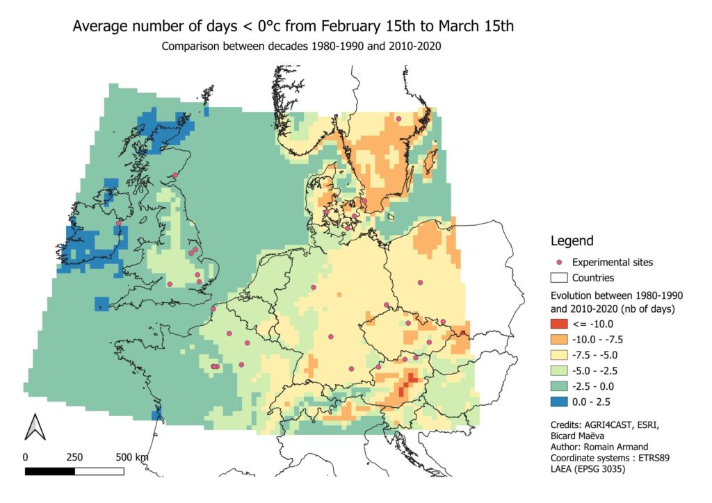
You are expected to design a map that shows the evolution of the average number of days with mean air temperature < 0°C between February 15th and March 15h. This period roughly corresponds to the emergence and tillering stages. The map should compare 2 decades: 1980-1990 and 2010-2020 to visualize the impact of climate change on temperatures.
Below is an example of the expected map. The map should use the coordinate system ETRS89 LAEA (EPSG Code 3035).
4. Dataset
The dataset can be downloaded here .
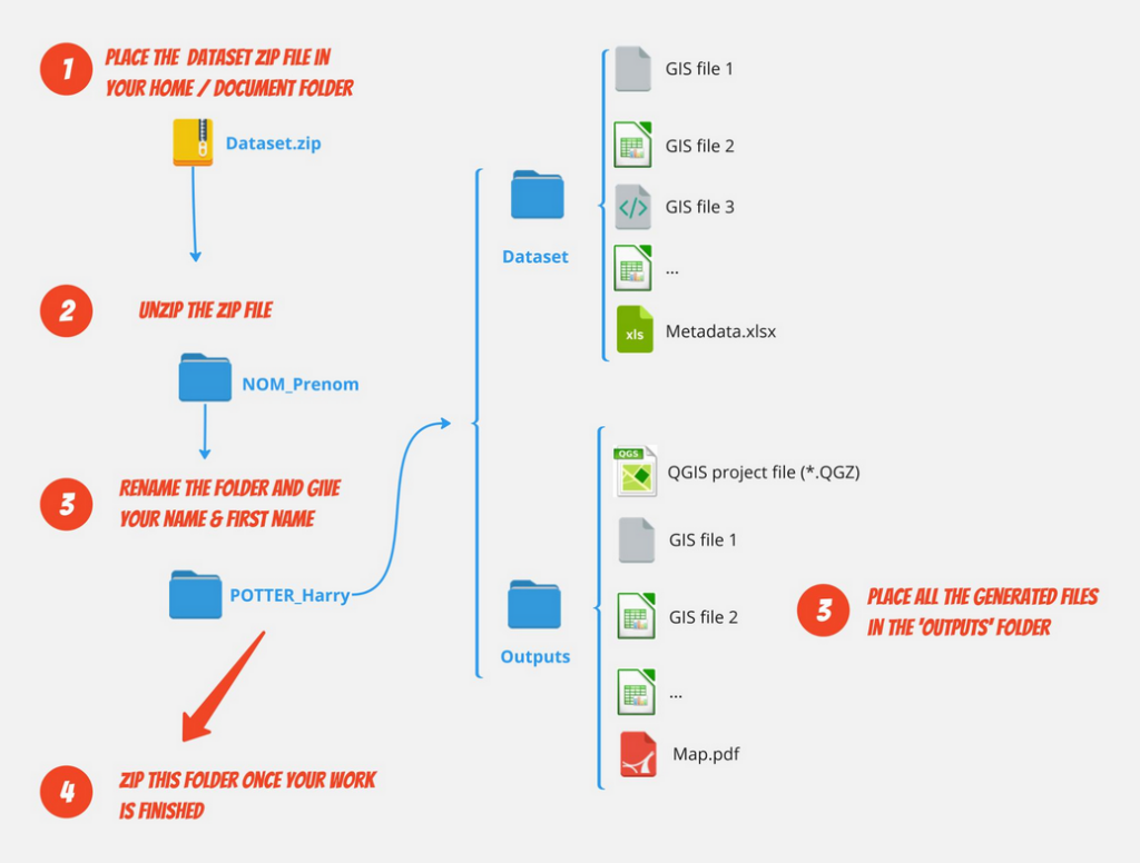
Follow the guidelines below to organise your dataset. All the generated files must be placed in the ‘Output‘ folder.
Focus on the dataset
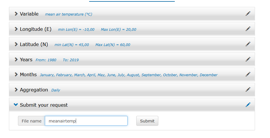
The climatic data will be based on the AGRI4CAST Resources Portal. Agri4Cast is a system developed by the European Commission’s Joint Research Centre (JRC) providing accurate and timely crop yield forecasts and crop production biomass for the European Union. The system integrates remote sensing, meteorological observations, agro-meteorological modeling, and statistical analysis tools to monitor and forecast crop growth and yield.
It includes minimum and maximum temperatures (°C), sum of precipitations (mm day−1) and total solar radiation (MJ mm−1 day−1). The dataset can be downloaded freely.

The meteorological dataset is composed of NetCDF (Network Common Data Form) files. This file format is used for storing multidimensional scientific data. It is widely used in fields such as climatology, meteorology, oceanography, and other geosciences. The common dimensions are time, longitude, latitude and climatic variables. In this exercise, the climatic data have been extracted on a daily basis.
5. R analysis
Step 1: Explore the metadata of the netcdf file
Create a new R project and a new R script. Copy and paste the script below in the script.
install.packages("ncdf4") #installation du package permettant la lecture du netcdf

library(ncdf4) #activation du package


nc_file <- nc_open("mean_air_temp.nc") # à paramétrer selon votre organisation de données
print(nc_file)  # Affichage des métadonnées

# Extraire les valeurs des dimensions
time <- ncvar_get(nc_file, "time")
lon <- ncvar_get(nc_file, "lon")
lat <- ncvar_get(nc_file, "lat")

# Vérifier les tailles du dataset
length(time)  # 14 926 (nb de jours)
length(lon)   # 95 (nb de lignes dans le raster)
length(lat)   # 47 (nb de colonnes dans le raster)


# Convertir le temps en format Date
time_origin <- as.Date("1978-12-31") #prendre en compte l’unité "days since 1978-12-31" :
time_dates <- time_origin + time


# Obtenir la première et la dernière date
first_date <- min(time_dates)
last_date <- max(time_dates)

# Afficher les résultats
print(first_date)
print(last_date)
Step 2: Visualise the first day of the netcdf file with ggplot
Create a new R script. Copy and paste the script below in the script.
# Si nécessaire installer les bibliothèques ci-dessous.
# Charger les bibliothèques nécessaires
library(ncdf4)
library(ggplot2)
library(dplyr)
# Ouvrir le fichier NetCDF
file_path <- "mean_air_temp.nc" # à paramétrer selon votre organisation de fichiers
nc_data <- nc_open(file_path)
print(nc_data)
# Extraire les dimensions
lon <- ncvar_get(nc_data, "lon")
lat <- ncvar_get(nc_data, "lat")
time <- ncvar_get(nc_data, "time")
# Convertir le temps en dates
origin <- as.Date("1978-12-31")
dates <- origin + time
# Extraire la variable de température moyenne
mean_air_temp <- ncvar_get(nc_data, "AirTemperatureMean")
# Remplacer les valeurs manquantes (-999) par NA
mean_air_temp[mean_air_temp == -999] <- NA
# Extraire la température pour le premier jour
mean_air_temp_day1 <- mean_air_temp[, , 1] # 1er jour (index 1)
# Convertir les données en un data frame pour ggplot
temp_data <- expand.grid(lon = lon, lat = lat) # Créer une grille avec lon et lat
temp_data$temp <- as.vector(mean_air_temp_day1) # Ajouter la température à chaque point
# Visualiser avec ggplot2
ggplot(temp_data, aes(x = lon, y = lat, fill = temp)) +
geom_tile() + # Créer une carte avec des tuiles
scale_fill_viridis_c(option = "C", na.value = "grey") + # Ajouter une échelle de couleurs (viridis)
theme_minimal() + # Thème minimal
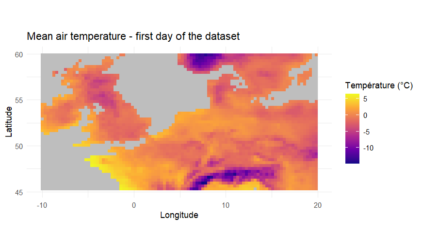
labs(title = "Mean air temperature - first day of the dataset", x = "Longitude", y = "Latitude", fill = "Température (°C)") +
coord_fixed(ratio = 1) # Garder un ratio fixe pour que la carte soit proportionnelle
You should be able to obtain this map preview.
Step 3: Calculate the number of days < 0°c between February 15th and March 15h
# Si nécessaire installer les bibliothèques ci-dessous.

#Activation des bibliothèques
library(ncdf4)
library(terra)

# Ouvrir le fichier NetCDF
nc_file <- nc_open("mean_air_temp.nc")# à paramétrer selon votre organisation de fichiers

# Extraire les variables
time <- ncvar_get(nc_file, "time")  # Temps
temp_data <- ncvar_get(nc_file, "AirTemperatureMean")  # Température moyenne
lon <- ncvar_get(nc_file, "lon")  # Longitude
lat <- ncvar_get(nc_file, "lat")  # Latitude

# Fermer le fichier
nc_close(nc_file)

# Convertir les temps en dates
time_origin <- as.Date("1978-12-31")  # Origine du temps
time_dates <- time_origin + time  # Conversion en dates

# Définir les périodes des décennies
decades <- list(
  "1980-1990" = c(as.Date("1980-01-01"), as.Date("1989-12-31")),
  "1990-2000" = c(as.Date("1990-01-01"), as.Date("1999-12-31")),
  "2000-2010" = c(as.Date("2000-01-01"), as.Date("2009-12-31")),
  "2010-2020" = c(as.Date("2010-01-01"), as.Date("2019-12-31"))
)

# Créer un dossier de sortie s'il n'existe pas
output_dir <- "output_raster"
if (!dir.exists(output_dir)) {
  dir.create(output_dir)
}

# Créer une liste pour stocker les rasters
raster_list <- list()

# Boucle sur chaque décennie
for (decade in names(decades)) {

  # Définir la période
  start_decade <- decades[[decade]][1]
  end_decade <- decades[[decade]][2]

  # Filtrer les indices des dates correspondant à cette décennie et la période 15/02 - 15/03
  date_filter <- which(
    time_dates >= start_decade & time_dates <= end_decade &
      format(time_dates, "%m-%d") >= "02-15" & format(time_dates, "%m-%d") <= "03-15"
  )

  # Extraire les températures correspondant aux dates filtrées
  filtered_temps <- temp_data[,,date_filter]  # Garde toutes les longitudes/latitudes

  # Vérifier si les données sont bien numériques avant de continuer
  if (is.numeric(filtered_temps)) {
    # Compter le nombre de jours où la température est < 0°C pour chaque pixel (lon/lat)
    cold_days_count <- apply(filtered_temps, c(1,2), function(x) sum(x < 0, na.rm = TRUE))

    # Créer un raster avec `terra` en WGS84
    r <- rast(nrows=length(lat), ncols=length(lon), xmin=min(lon), xmax=max(lon), ymin=min(lat), ymax=max(lat))
    values(r) <- as.vector(cold_days_count)

    # **Définir le système de coordonnées initial en WGS84 (EPSG:4326)**
    crs(r) <- "EPSG:4326"

    # **Inverser les latitudes (axe Y)**
    r <- flip(r, direction = "vertical")

    # **Reprojection en EPSG:3035**
    r_proj <- project(r, "EPSG:3035")

    # Ajouter le raster reprojeté à la liste
    raster_list[[decade]] <- r_proj

    # Définir le chemin de sortie
    output_path <- file.path(output_dir, paste0("cold_days_", decade, ".tif"))

    # Exporter le raster reprojeté en GeoTIFF
    writeRaster(r_proj, filename=output_path, filetype="GTiff", overwrite=TRUE)

  } else {
    warning(paste("Les données de température pour la décennie", decade, "ne sont pas numériques"))
  }
}

# Afficher un raster en aperçu (par exemple pour la décennie 1980-1990)
if ("1980-1990" %in% names(raster_list)) {
  plot(raster_list[["1980-1990"]], main="Nb jours < 0°C du 15/02 au 15/03 (1980-1990)")
} else {
  warning("Le raster pour la décennie 1980-1990 n'a pas été généré.")
}
Chek out you working dataset. A folder named ‘output_raster’ should have been created. It should contain TIFF raster that can be loaded into QGIS.