Learning from the daily errands of GPS tagged European hares
1. About this exercise
The data and study case for this practical are based on the work of Mayer et al, 2023 .
- GIS expertise: intermediate
- Duration : 3 hours
- GIS software: QGIS 3
- Last update: 2024
- Author: Chloé Girka
2. Context
Roads transform landscapes. On the one hand, they form a dangerous obstacle. On the other hand, their verges provide ressources for local animals. In their research, Meyer et al investigated the impact of the road network on space use by the European hare (Lepus europaeus). To achieve this goal, they analyzed data from 90 tagged hares living in three different parts of Europe: Denmark, Northern Germany and Southern Germany.
We will use the data from this research as an opportunity to learn about animal tracking data analysis, landscape metrics, and automatisation in QGIS. And because spatial data is data, you will be able to export it to perform statistical analyses.
3. Theorical background
a. Home range computation
The home range is the area used by an animal for its activities. It can be determined using the animal’s GPS coordinates. There are different methods to compute home range.
The simplest method is to build the smallest possible convex polygon around all locations. This method is available in QGIS and requires no external plugin. However, since this method takes all points into account, it tends to overestimate the home range.
Other methods have been developped, which ignore locations that were the least visited. Among these methods, the Restricted Minimum Convex Polygon is available in QGIS through the AniMove plugin.
b. Landscape metrics
Landscape metrics are used to quantify landscape patterns. Over the past decades, hundreds of them have been developped. They describe a range of aspects: area and edge, shape, core area, contrast, aggregation, diversity… We will compute a few metrics based on formulas found in the FragStats documentation .
4. Instructions
a. Working environment
Dataset
Coordinate system
This project takes place in Germany. We will use the coordinate system ‘WGS 84 / UTM zone 32N‘ (EPSG: 32632).
Metadata review
You will find three vector datasets and a table:
- Hare_raw_data: GPS tracking data of all the hares. The geopackage format allows to store date and time data.
- Landcover_AOI: Photo-interpreted land cover, used as a proxy for habitats.
- Road_network_OSM: Road network extracted from OpenStreetMap.
- Hare_additional_info: Additionnal information about individual hares: their sex and the study area they belong to.
Answer the following questions about the datasets:
- How many different hares do we have data about? What are their names?
- What is the time span of the dataset?
- What is the coordinate system of the GPS tracking data?
- What are the different landcover classes?
Step 1: Preparing the hare data
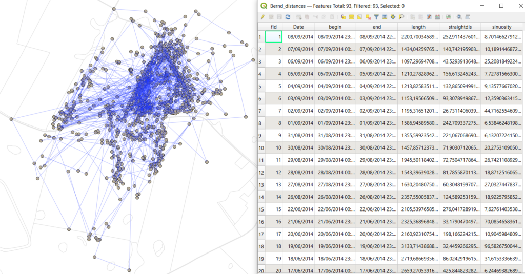
Step 2.1. Bernd’s daily whereabouts
Bernd is our first hare. We want to know Bernd better. First, let’s look at the distances it travels everyday. Using the following elements, can you build a workflow to see Bernd’s movement everyday as well as the travelled distance?
You can test out the workflow in QGIS.
Step 2.2. Automation
Bernd is one of many hares. Maybe its behaviour is different from that of its fellow hares. Is Bernd lazy? Hyperactive? Average?
If we want to compare Bernd’s data to that of other hares, we need to repeat Step 2.1 for each hare. We will use QGIS’s Model Designer. It will allow us to combine several tools in one model.
Help yourself from this quick startup guide and copy the following model:
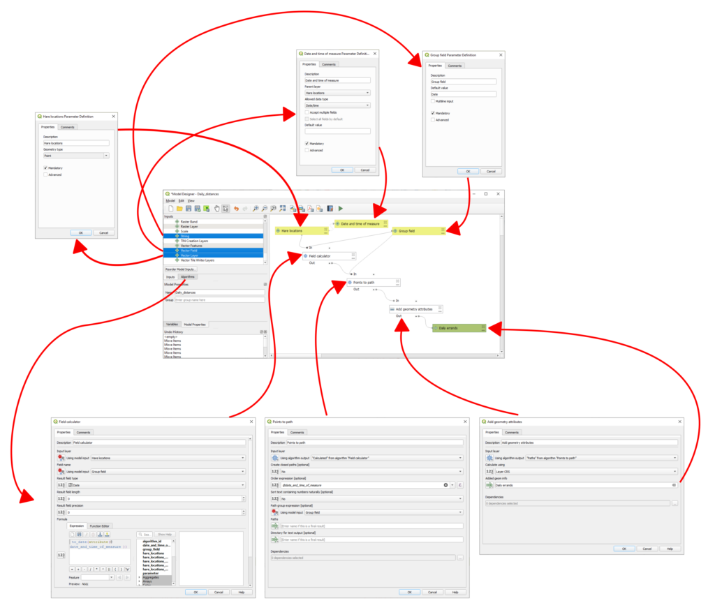
Once your model is ready, test it on Carlos’s tracking data.
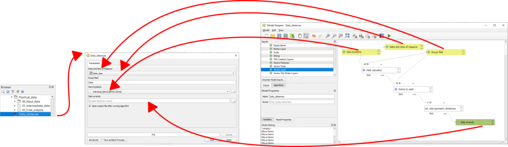
If the test is successful, move to the next step: batch processing .

To get all the data into a single file, merge the layers together.
Bonus: You can export the data to run statistical analyses in R.
Step 3.1. Home range
Ideally, we want to compute the home range of each hare using the AniMove plugin. However, installing it requires extra steps that may vary from computer to computer. To keep this practical simple, we will use QGIS’s built-in Minimum Bounding Geometry. The output contains an area field. Hence, there is no need to add geometry attributes.
Step 3.2. Landscape metrics: the patch approach
Many landscape metrics are based on patches: areas that share the same land cover or habitat. In this step, you will summarize information about the patch composition of each home range.
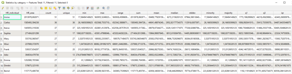
From this table, you can eithere directly read, or compute landscape metrics such as:
- Patch richness (PR) : « count »
- Total Area : « HR_area » / 10000
- Largest Patch Index (PI) : « max » / « HR_area »
Bonus 1.1. Road density
Road density is the total length of roads divided by the area of the home range. We will only focus on road types ‘motorway’, ‘primary’, ‘secondary’ and ‘tertiary’.
Try building a model for road density calculation. This model should take the home range(s) and main roads as input, and return a table that contains the road density of the home range(s).
Bonus 1.2. Road avoidance
One of the questions from Mayer et al.’s original research was: Do hares avoid roads?
To try answering this question, we can compare the road density of the real home range to that of a theoretical circular home range of the same surface area.
To compute this theoretical home range, we need:
- a center, calculated as the mean coordinates of each hare’s locations;
- a radius, derived from the formula to calculate’s a disk area: Area = π * Radius²
Bonus 2: Statistical analysis
If you are ahead of time, you can gather all your data into one table and export it for further analysis in R.
Try answering the following questions:
- Is there a difference in road density between real and theoretical home ranges?
- Is there a significant difference in home range sizes? among individuals? between Northern and Southern Germany? between males and females?
- Is there a significant difference in daily movements? among individuals? between months?